Motion Estimation for Video Processing
Contents
All methods described here are for natural images and are unlikely to work well with synthetic images.
Global Motion Estimation
Introduction
Phase correlation is one technique that can be used to find the global alignment between two images quickly. This is an example of direct motion estimation because it operates directly on the pixel values.
Images are transformed to the frequency domain, therefore a window must be applied to the images to avoid the edges from correlating and resulting in zero motion. Unfortunately, the windowing reduces the maximum amount of motion that can be measured.
The output of phase correlation is a surface where conveniently the height represents the confidence and the location represents the motion.
Phase correlation is usually used to find translation but can be extended to find rotation and scale. For other motion models it is possible to use pixel difference gradients to optimise the motion model. If there is a lot of local motion or depth in the scene then indirect motion estimation using features can be better.
Pros
- Large search range and evaluates every position simultaneously
- Simple search to find the global maximum
- The correlation surface can be interpolated to obtain subpixel motion
- Fast - uses the FFT of which there are optimised implementations, such as FFTW for CPU or cuFFT for GPU
Cons
- The need for windowing reduces the search range
- Moving objects in the scene may reduce the global correlation peak resulting in reduced confidence
Implementation
- Load the images and convert to luminance (or grey)
- Apply windowing
- Compute the phase correlation surface and find the location of the peak
Example
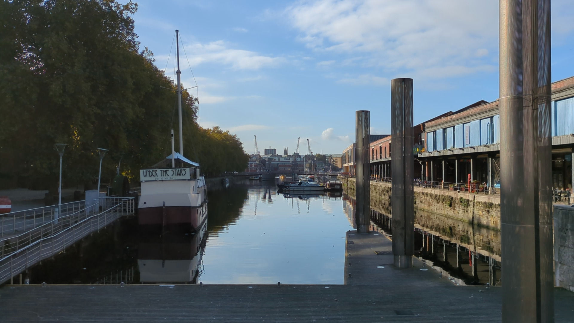
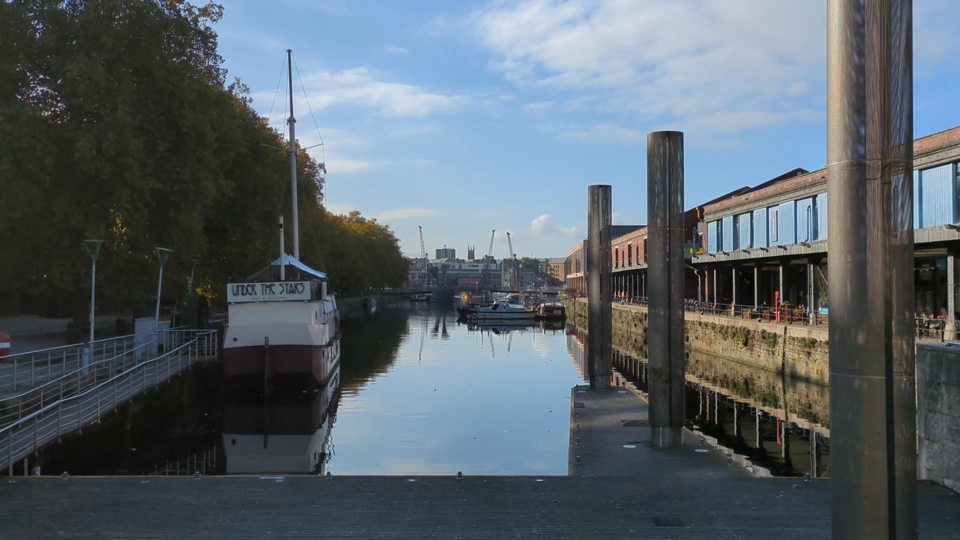
These are 2 images that we will will use to test our approach with, the camera was panning to the right in this shot and the images are 5 frames apart:
Calculate the phase correlation between these 2 images:
pc.py --current frame_00160.png --previous frame_00155.pngThis produces the following output:
Detected shift: (14.143573237407736, -0.13359329274885567), Correlation: 0.8721376508547936Composite the 2 images into the same co-ordinate frame:
globalmc.py --current frame_00160.png --previous frame_00155.png --xoff 14.143573237407736 --yoff -0.13359329274885567 --outline --output aligned.pngHere is the composited output:
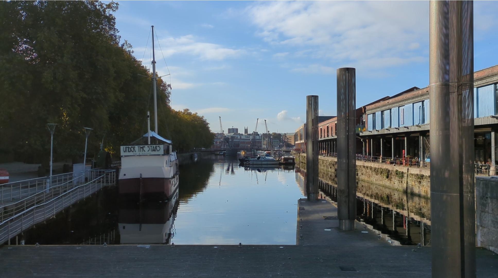
Using the --outline parameter draws a yellow box around the previous image (you may have to zoom to see it). It's a pretty good result for non-consecutive images. All the detail from the image on the right are visible on the right edge and on the left edge there is detail added from the left image.
Some discontinuities can be seen at the edges of combined images due to rotation of the camera, lens distortion. objects at different depths in the scene (parallax) and local object motion. Other methods may use motion or camera models that can account for these effects.
An alternative method would be to use feature detection and matching for indirect motion estimation. An implementation is provided in the gfm tool; motion vectors are obtained using the position of each feature point and its matching position in the other image. The median motion vector is found to avoid bad matches and other outliers. Results from that method are comparable.
Summary
- Phase correlation is fast
- Limited ability to represent complex motion and depth
- Simple implementation - only two function calls in OpenCV after loading images and getting them into a suitable format
Local Motion Estimation
Introduction
Local motion estimation is a core algorithm for video compression via motion compensation and residual encoding. Block matching algorithms divide frames into a grid of blocks and search for matches in another frame. This method is used in video coding standards such as MPEG-4/H.264, HEVC/H.265 and VVC/H.266.
Pros
- Detailed local motion, can handle dynamic scenes and parallax
- Motion field can approximate more complex global motion models
- The motion field is a compact representation that given a previously decoded image can approximate the next image in a sequence
Cons
- Computationally expensive, some block matching algorithm strategies can speed up the search
- Difficult to find motion at image borders
- Not guaranteed to be "true" motion; must be further processed if not for video compression
Implementation
- Load "current" and "previous" images
- Convert to luminance/grey
- Divide current image into blocks
- For each block search for best match in the previous image
- Sub pixel motion refinement around best integer vector
There are many choices for the block search algorithm, usually resulting in a trade off between image quality and speed. Selection is determined by whether the algorithm will be implemented in software, ASIC or FPGA and whether it is needed for offline or online use.
There are 2 algorithms implemented here: the two dimensional full search (2DFS), a brute force approach and PMVFAST, an algorithm that uses predictors based on spatio-temporally neighbouring blocks, the median vector and early search termination combined with small or large diamond search patterns.
In the PMVFAST paper we can infer that the authors use a block size of 16×16 pixels and the threshold values they give are based on this size. In modern video coding standards blocks can be other sizes and can also be subdivided.
Example
Using the full search, find the motion vectors between two images; apply motion compensation to produce a prediction of the current image using only the previous image:
bma -c current.jpg -p previous.jpg -v motion.mv
bmc -p previous.jpg -v motion.mv -o compensated_current.jpg
Using PMVFAST, find the motion vectors:
bma -c current.jpg -p previous.jpg -a pmvfast -v motion.mvUsing the provided evaluation script, evaluate.py,
we can generate the motion vectors and motion compensated frames from the video
below. The actual video tested (preview below) was 1920×1080, 385 frames
at 30 fps and the block size was set to 8×8. Use of temporal neighbours
was not implemented in PMVFAST and both methods could have been accelerated
by using SIMD and multithreaded programming techniques.
Video Sequence Used for Testing
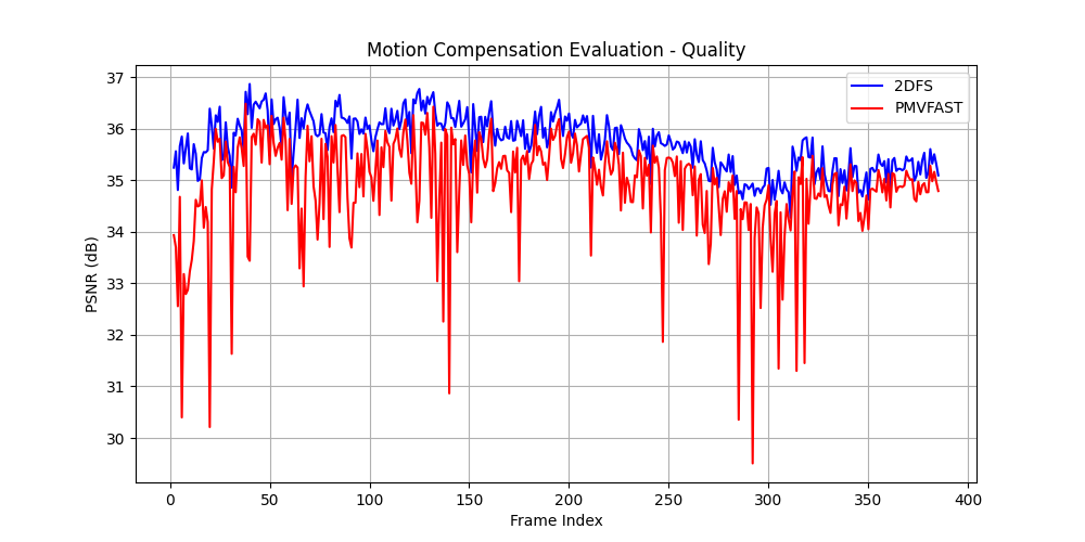
| Method | Average PSNR (dB) | Average Time (secs) |
|---|---|---|
| 2DFS | 35.72 | 30.5 |
| PMVFAST | 34.91 | 0.28 |
Peak Signal to Noise Ratio (PSNR) is a metric for comparing images. Above 30 dB it becomes more difficult to spot artefacts. Above 40 dB you usually need to zoom to find artefacts and compression noise (during capture) and sensor noise are at a similar scale to motion estimation artefacts.
Most of the artefacts visible in the motion compensated video are at the edges of the frame, i.e. not possible to compensate from motion alone.
Despite PMVFAST dropping in quality at various times; almost all frames were recovered at greater than 30 dB. In a video codec, residual coding will make up for poor motion vectors and edge effects; furthermore, a rate-distortion mechanism will trade off quality to achieve the desired bit rate for the final video stream.
Summary
- PMVFAST was 100 times faster at the cost of less than 1 dB of quality, on average
- Reduced search algorithms, such as PMVFAST can give impressive results but will not beat 2DFS
- In silicon based implementations it may be worthwhile to simply use 2DFS
Optical Flow Estimation
Introduction
Optical flow describes the apparent 2D motion of pixels in a video frame and is useful for motion segmentation, tracking and video completion. There are several methods for estimating per-pixel motion, the simplest method would be to match a neighbourhood of pixels surrounding a central pixel with a similar neighbourhood in another frame. Optical flow methods use additional constraints, with the main being that the change in intensity of a moving pixel corresponds to the amount of motion in (x,y) and the amount of time that has passed.
Pros
- Very detailed local motion
- Good starting point for frame rate upsampling or for motion segmentation
Cons
- Aperture problem
- Storage of optical flow field is not compact
Implementation
- Load current and previous images
- Convert to luminance/grey
- Estimate optical flow, using top level API or inference
- Visualise flow using colour
OpenCV implements Farnebäck's polynomial expansion based method for optical flow estimation. It matches polynomials fitted to local neighbourhoods of pixels. A global motion model is fitted under the assumption that local flow vectors vary slowly to aid robustness and the algorithm is run at multiscale to support large displacements.
RAFT (Recurrent All-Pairs Field Transforms) is a deep model for optical flow estimation. As the name suggests, the method matches all pixels in one image to all possible matches in the second image. Despite the computational cost, speed is kept high by working on downsampled features, re-using the all-pairs correlation, efficient refinement of flow vectors and GPU implementation.
Example
For testing, frames 150 and 149 of the Basketball sequence [*] will be used:
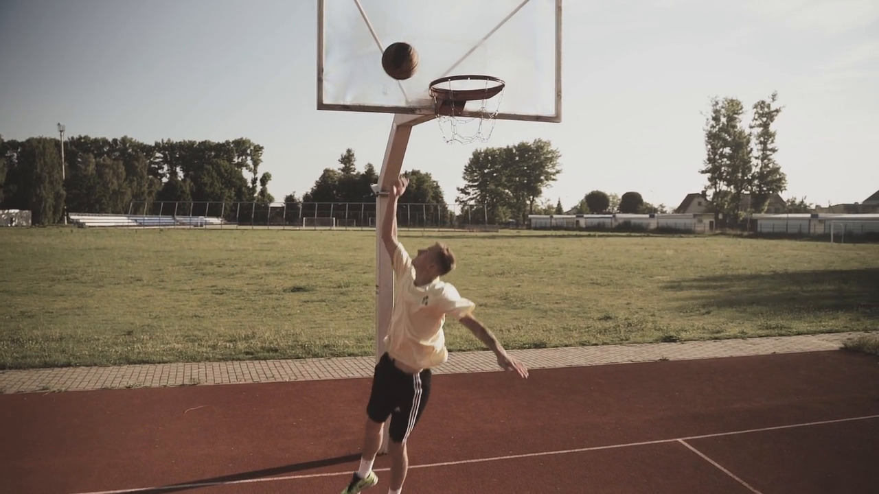
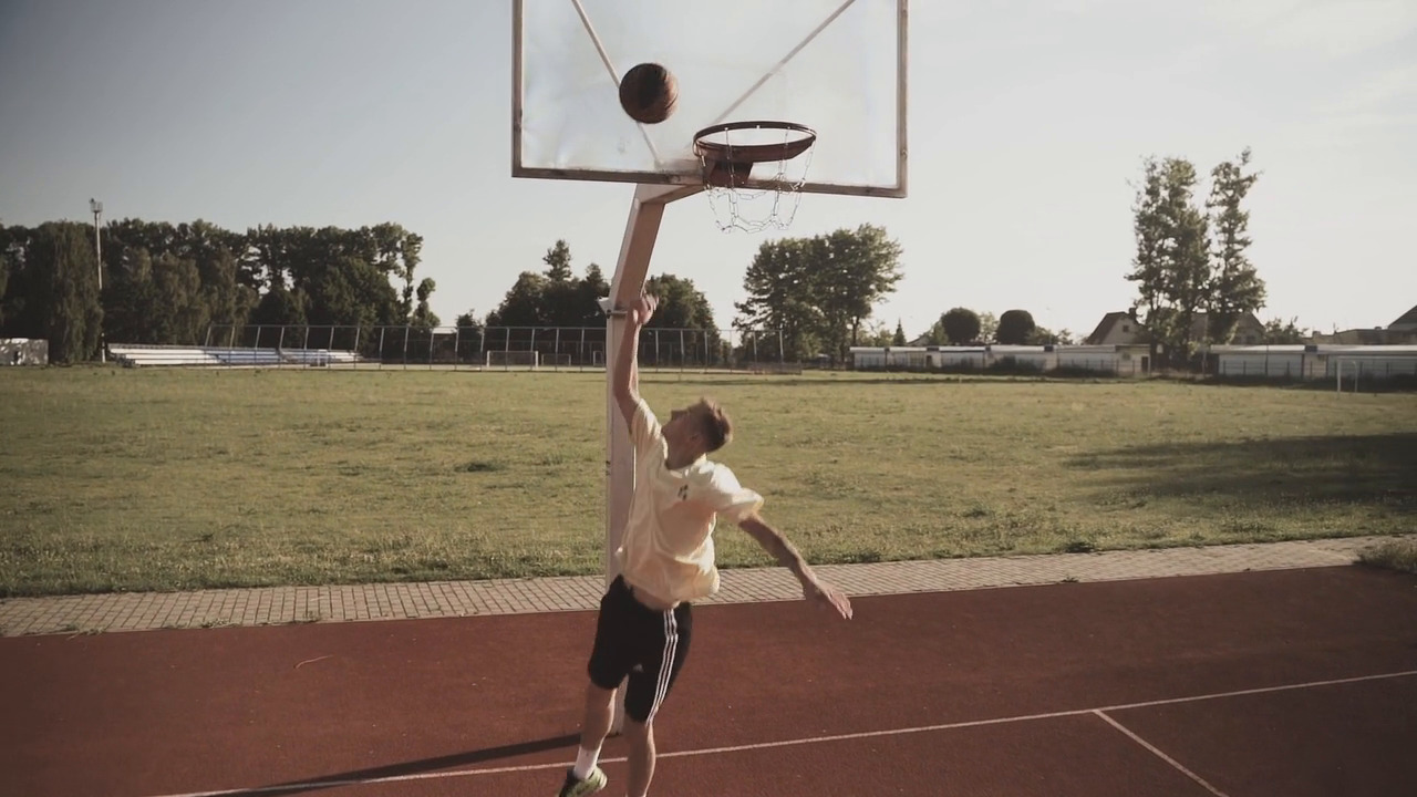
Using OpenCV's impementation of Farnebäck's method, find the optical flow between the two images:
ocv-of-single.py --current frame_00150.png --previous frame_00149.png --output flow-visualisation.pngThe optical flow result:
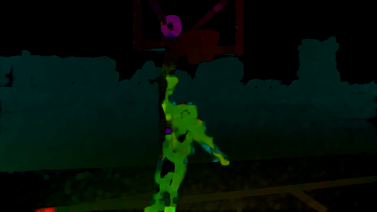
Optical Flow estimated using Farnebäck's method
In this visualisation of the optical flow vectors, the colour corresponds to the direction and the brightness corresponds to the vector magnitude.
You can extract all images from a video to a directory, compute optical flow for all consecutive image pairs, and save images visualising the flow using this script:
ocv-of-sequence.py --video input.mp4 --images extracted_frames --flow flowImages from the video will be saved into the extracted_frames directory and visualisation images into the flow directory:
PyTorch contains the RAFT model in the torchvision module. To use RAFT, we must,
- Get the RAFT model and weights from torchvision
- Load the images into PyTorch tensors
- Preprocess images by resizing to 960×520 (no need to convert to grey)
- Use the model to predict the flow
This is implemented in Python based on the PyTorch tutorial for RAFT;
two scripts process either a single pair of frames or a video
sequence. The scripts are raft-of-single.py and
raft-of-sequence.py. They take the same
parameters as the OpenCV scripts above.
Here is the optical flow estimated for the same Basketball images,
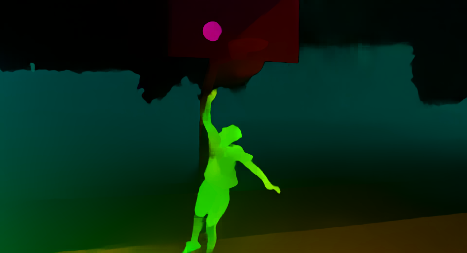
Optical Flow estimated using RAFT
Although this result looks better, we need to compare in an objective way. To make a comparison between Farnebäck's method and RAFT, frame 149 from the basketball sequence was compensated using the optical flow and PSNR was calculated against frame 150.
As RAFT estimates flow at a lower resolution (960×520) to the source video (1280×720), the PSNR was computed after resizing the image.
The compensated image was resized using ImageMagick convert, i.e.
convert -resize 1280x720! compensated.png compensated_1280x720.png| Method | PSNR (dB) |
|---|---|
| Farnebäck | 38.3183 |
| RAFT | 31.8379 |
The flow from the whole sequence was also computed, as previewed below.
Optical Flow for the Basketball Sequence
Summary
- RAFT estimates optical flow at a reduced resolution and it was faster to estimate
- Farnebäck's method only required one function call after loading images and getting them into a suitable format; RAFT also required downloading the model, weights and setting up transforms
References
- B.S. Reddy and B.N. Chatterji, "An FFT-based Technique for Translation, Rotation, and Scale-Invariant Image Registration", IEEE Transactions on Image Processing, vol. 5, issue 8, pp 1266-1271, DOI 10.1109/83.506761, 1996
- A.M. Tourapis, O.C. Au and M.L. Liou, "Predictive Motion Vector Field Adaptive Search Technique (PMVFAST) - Enhancing Block Based Motion Estimation", Proceedings of SPIE - The International Society for Optical Engineering, DOI 10.1117/12.411871, 2001
- G. Farnebäck, "Two-Frame Motion Estimation Based on Polynomial Expansion", Scandinavian Conference on Image Analysis (SCIA), DOI 10.1007/3-540-45103-X_50, 2003. pdf
- Z. Teed and J. Deng, "RAFT: Recurrent All-Pairs Field Transforms for Optical Flow", European Conference on Computer Vision (ECCV), DOI 10.1007/978-3-030-58536-5_24, 2020. pdf
Credit
Basketball sequence from pexels.com, by Pavel Danilyuk, downloaded via PyTorch.