Introduction

In recent years radiance field methods have been a hot topic in novel view synthesis; primarily Neural Radiance Fields (NeRFs). Quality has improved massively as NeRFs allow complex view dependent reflection effects when creating novel views. The drawbacks of NeRFs is that they require neural networks to be trained and rendering is slow.

More recently Gaussian Splatting has become the method of choice; with the advantages of a more compact scene representation, faster optimisation of the model and fast rendering while maintaining support for directional based appearance.

A Gaussian Splat is essentially an oblong represented by location (x,y,z) and covariance that defines how long and flat or wide and spherical it is. Colour and transparency are key parameters and spherical harmonics are used to represent view dependent colour properties.

Implementation

Most splatting algorithms work as follows:

1. Load a sparse point cloud
2. Initialise splats at each 3D point in the point cloud
3. Iterate:
   • Optimise all splats using photometric loss against images, to adjust size, shape and colour
   • Every N iterations: densify (add more splats in areas that need them), remove redundant splats (typically very small splats, splats that have high transparency or splats that are co-located with more dominant splats)
4. Export splats in a file

The workflow is as follows:

1. Perform a sparse reconstruction with COLMAP (or SLAM or other reconstruction method and create a COLMAP project with the results)
2. Run a splatting algorithm using the COLMAP project and your images
3. View the splats; clean up if necessary

Splatting algorithms tend to take from about 15 minutes to an hour depending on the number of images, resolution and the scene. To generate a splat model, somewhere from 16 to a couple of thousand of images are required, depending on the resolution of the images, the camera poses and the size of the model, similar to a 3D reconstruction from more traditional techniques.

In this demonstration OpenSplat and gsplat will be used. OpenSplat is based on splatfacto which was based on the original 3DGS paper while gsplat implements multiple splatting algorithms.

The model from the reconstruction demo will be the basis for the splats that will be generated.

Example

Running OpenSplat

To build a docker image and run OpenSplat, first clone the repo:

git clone https://github.com/pierotofy/OpenSplat.git

Change directory to the freshly cloned repo and build the docker image,

cd OpenSplat
docker build -t opensplat --build-arg CUDA_VERSION=11.8 --build-arg TORCH_VERSION=2.7.1 .  

The CUDA and torch versions required modification in the docker build command in order to make it work with my system; you may need to change the above line.

Now run the docker image,

docker run  --gpus all -e NVIDIA_DRIVER_CAPABILITIES=compute,utility,graphics --rm -w /work -v "/data:/work" -it opensplat

I keep my COLMAP projects in the drive mounted at /data so you will probably have to change the above line to match where you keep your project data.

Then make a directory for your splats in your COLMAP project and run OpenSplat,

cd /work/path/to/colmap/project/
mkdir splats
/code/build/opensplat . -n 2000 -o splats/splat.ply

Setting 2000 iterations to build a splat is low and only for the purposes of previewing a model. You need closer to 30000 iterations to build a better quality model.

View the splats in SuperSplat: drag and drop the splat.ply file onto the web browser to view.

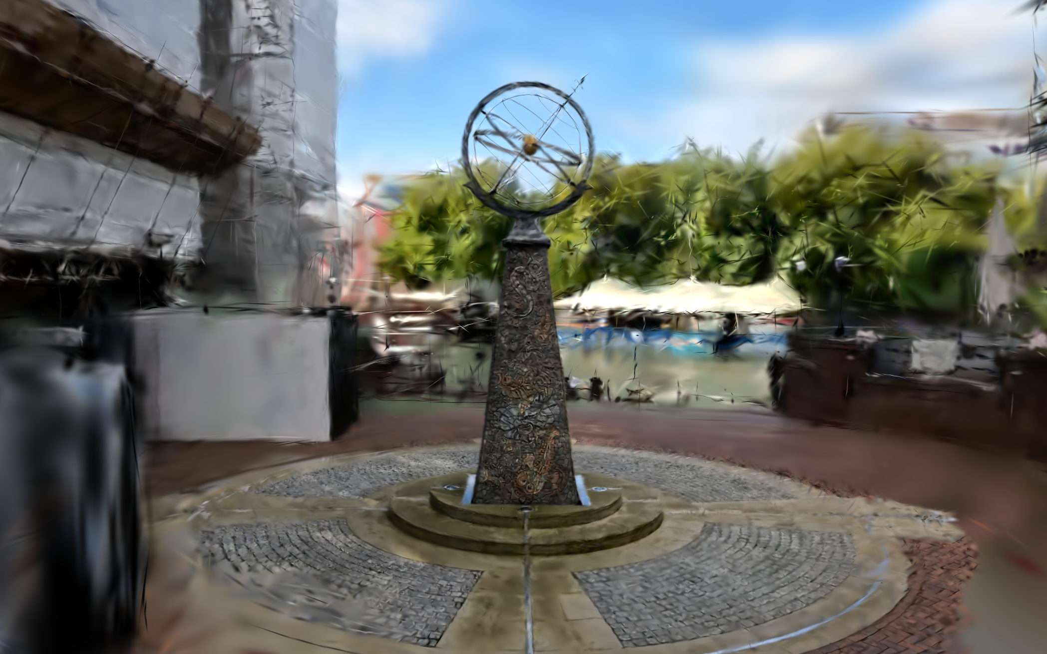
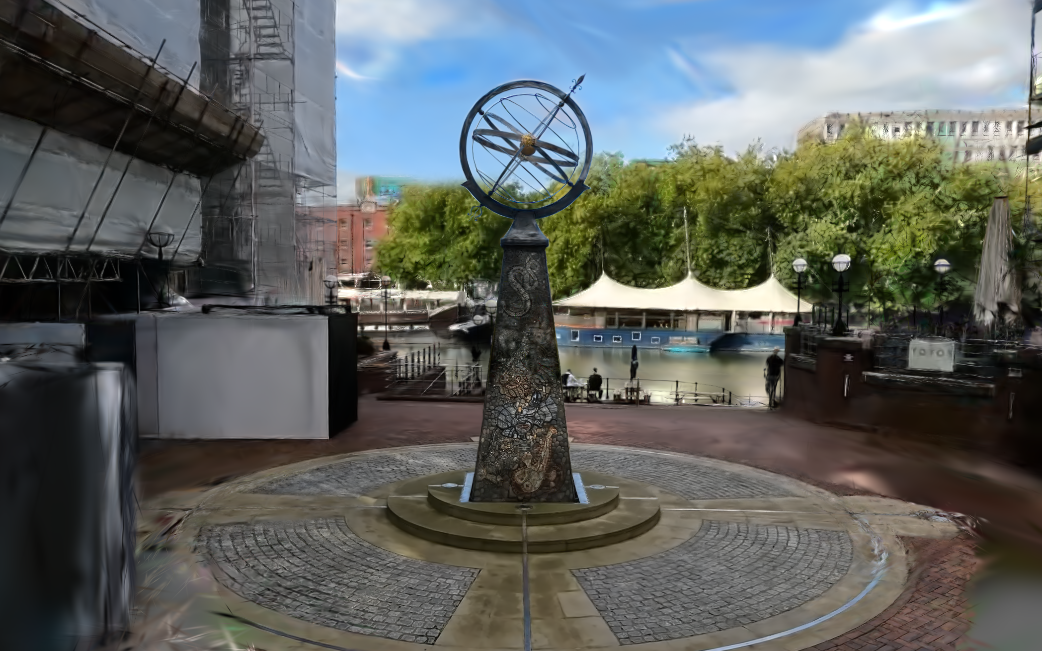
Click to see more detail; Left: 2000 iterations, Right: 30000 iterations

SuperSplat has some editing tools that are very handy for removing unwanted parts of the scene.

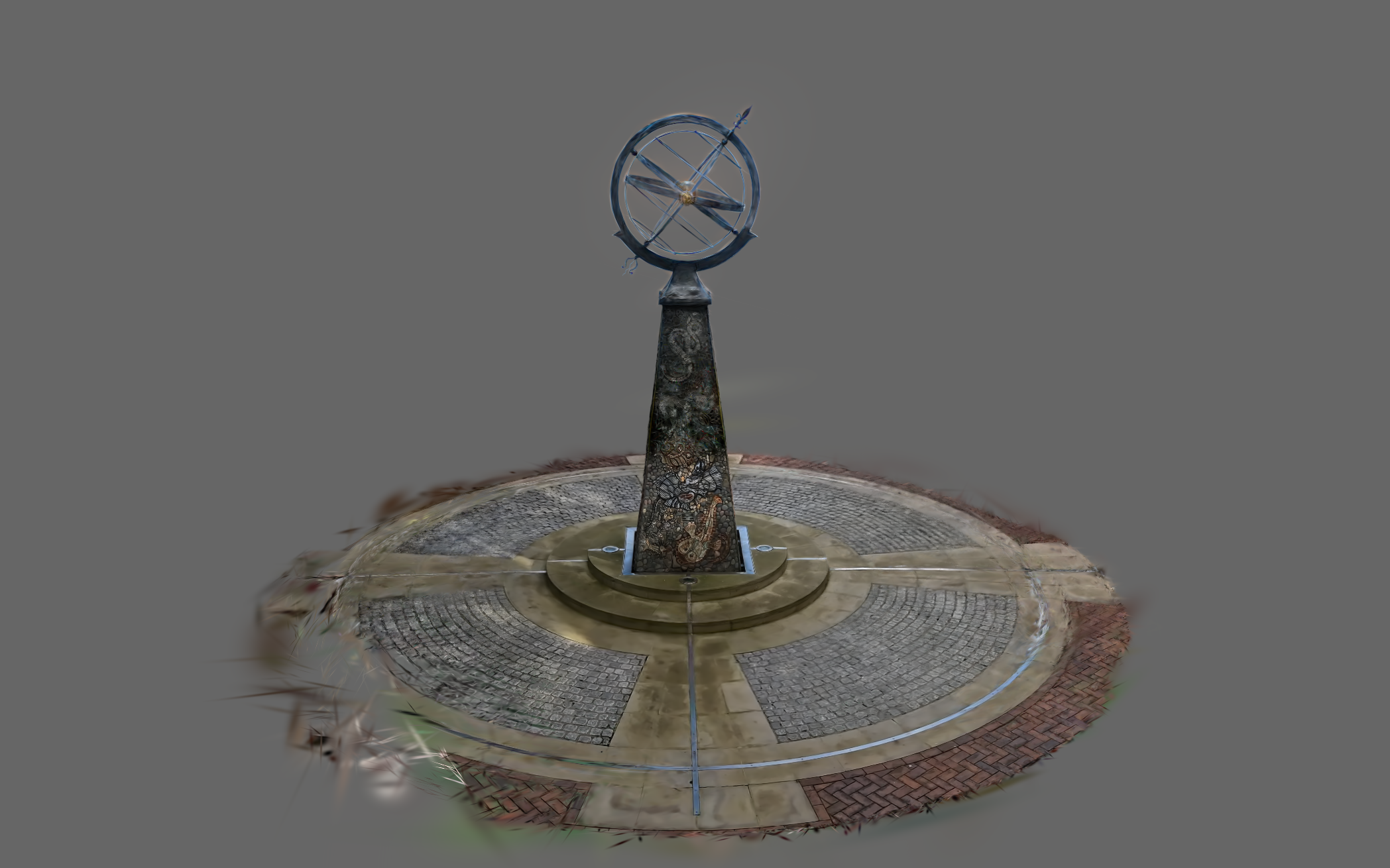
Exploration Statue Model

Splats viewed far from where images were captured do not look representative of the model

OpenSplat notes:

• OpenSplat only supports PINHOLE and SIMPLE RADIAL camera models; this is set during COLMAP feature detection.
• OpenSplat needs to load all your images into RAM so if you have too many images with too high a resolution then you may run out of memory.

Running gsplat

  Code on github

First, we are going to do some preparation for our COLMAP project using ImageMagick mogrify to create reduced resolution images to help gsplat.

cd /data/colmap/project_name
mkdir images_2
mogrify -resize 50\% -path images_2 images/*.jpg

Due to a bug in gsplat, it will resize the images again, but at least gsplat will run.

Use the gsplat.Dockerfile to build a docker image to run gsplat. Build and start the docker image on the working directory at /data,

rundocker.sh gsplat /data

Create a results directory for this project,

mkdir -p results/project_name

Start gsplat, running the Markov Chain Monte Carlo splatting algorithm (MCMC),

CUDA_VISIBLE_DEVICES=0 python ~/gsplat-1.5.3/examples/simple_trainer.py mcmc --data_dir /work/colmap/project_name/ --data_factor 2 --result_dir ../results/project_name --save-ply --ply-steps 20000

Optionally monitor the results in viser by opening a browser window to watch the splats being built although this can slow down the splatting. If you use the rundocker.sh script & gsplat docker image then viser will be running at http://localhost:8989/.

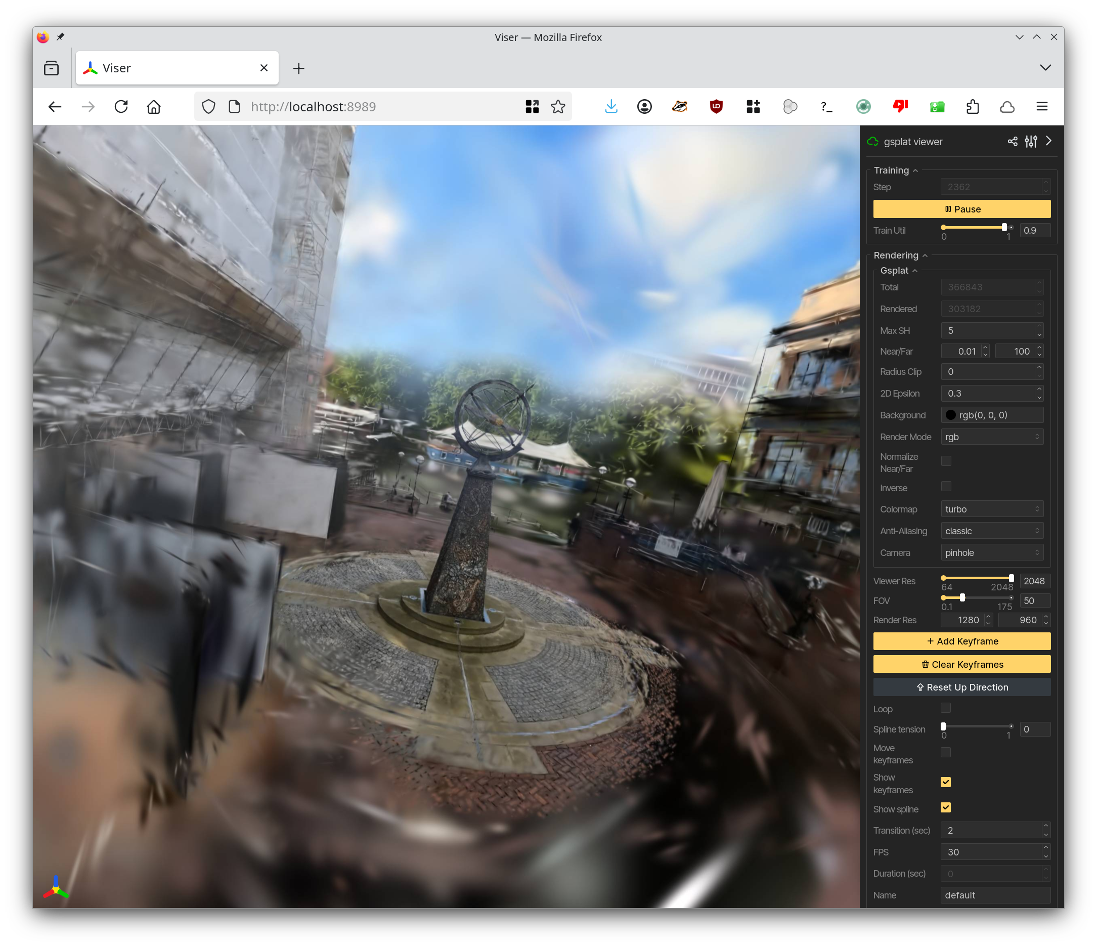
gsplat Training

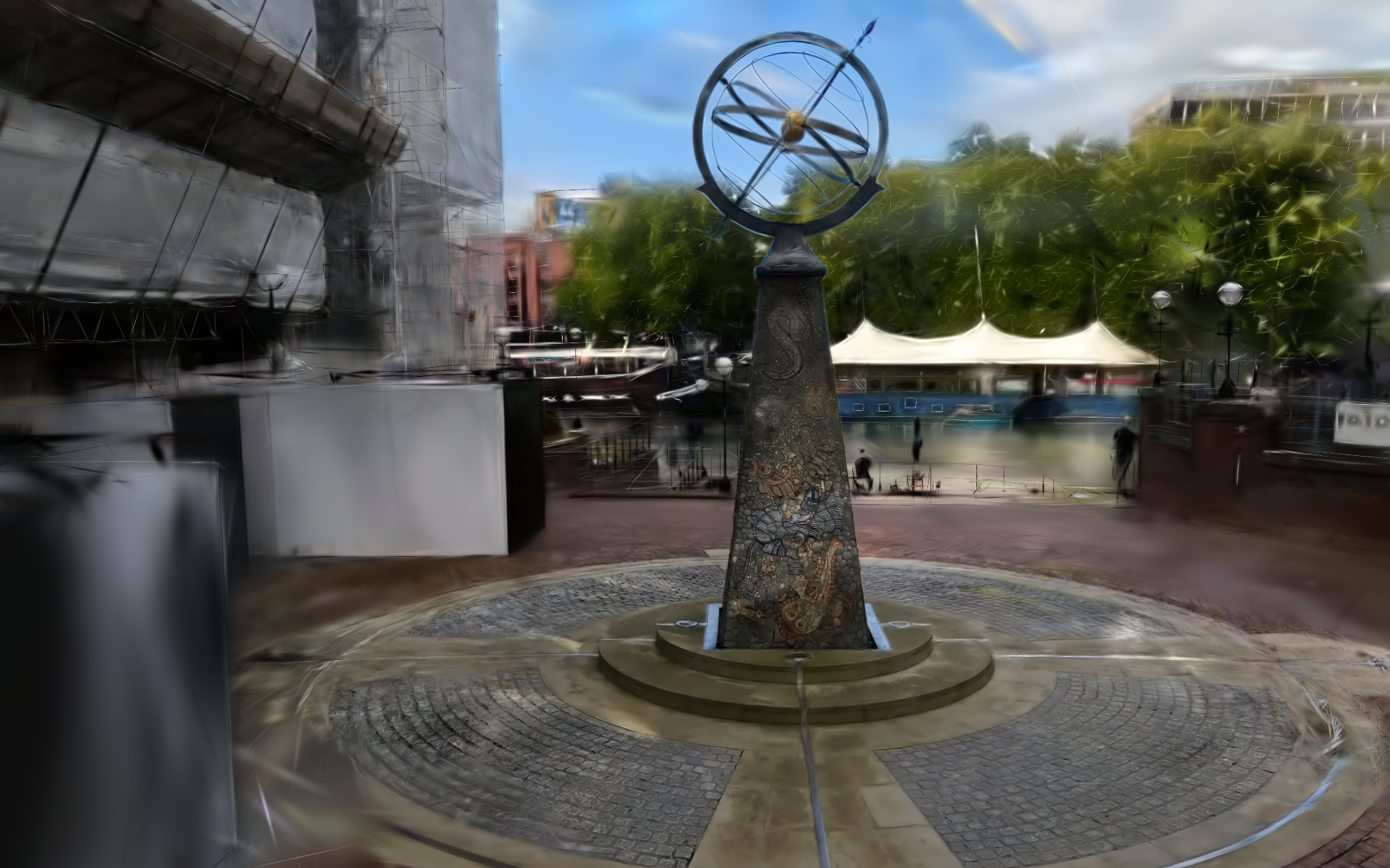
gsplat Result

Summary

• Splatting is a 3D modelling technique for novel view synthesis that is initialised from sparse reconstructions
• Splat models can achieve very high, photorealistic, quality
• Splat models look much better from viewpoints near to the actual camera positions

---

References

• Bernhard Kerbl, Georgios Kopanas, Thomas Leimkühler, George Drettakis, "3D Gaussian Splatting for Real-Time Radiance Field Rendering", ACM Transactions on Graphics, vol. 42, no. 4, 2023
• Shakiba Kheradmand, Daniel Rebain, Gopal Sharma, Weiwei Sun, Yang-Che Tseng, Hossam Isack, Abhishek Kar, Andrea Tagliasacchi, Kwang Moo Yi, "3D Gaussian Splatting as Markov Chain Monte Carlo", Advances in Neural Information Processing Systems (NeurIPS), 2024